Interpolation
Lagrange interpolation
Suppose that a list of \(m+1\) points \(\{(x_0, y_0),\dots,(x_{m}, y_{m})\}\) in \(\mathbb{R}^2\) is given, such that \(x_i\neq x_j\), if \(i\neq j\). Then
is a polynomial of degree m which passes through all the given points. Here
are Lagrange Basis Polynomials.
This procedure can be extended to multivariate case as well.
Suppose that a list of points \(\{{x}_1,\dots,{x}_{\rho}\}\) in \(\mathbb{R}^n\) and a list of corresponding values \(\{y_1,\dots,y_\rho\}\) are given. Let’s denote by \({\bf X}\) the tuple \(({\bf X}_1,\dots,{\bf X}_n)\) of variables and \({\bf X}_1^{e_1}\cdots{\bf X}_n^{e_n}\) by \({\bf X}^{\bf e}\), where \({\bf e}=(e_1,\dots,e_n)\).
If for some \(m>0\), we have \(\rho={{m+n}\choose{m}}\), then the number of given points matches the number of monomials of degree at most m in the polynomial basis. Denote the exponents of these monomials by \({\bf e}_i\), \(i=1,\dots,\rho\) and let
and for \(1\leq j\leq\rho\):
Then the polynomial
interpolates the given list of points and their corresponding values. Here \(|M|\) denotes the determinant of M.
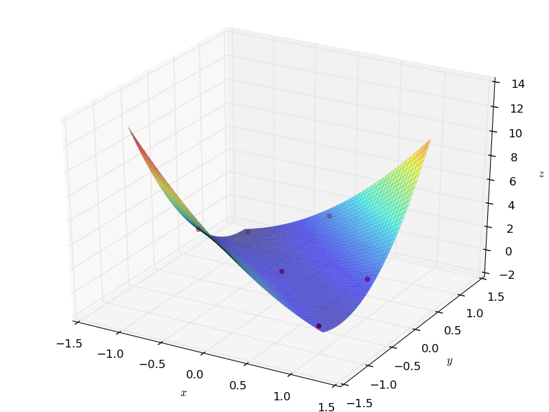
The above procedure is implemented in the Interpolation module. The following code provides an example in 2 dimensional case:
from sympy import *
from pyProximation import Interpolation
# define symbolic variables
x = Symbol('x')
y = Symbol('y')
# initiate the interpolation instance
Inter = Interpolation([x, y], 'sympy')
# list of points
points = [(-1, 1), (-1, 0), (0, 0), (0, 1), (1, 0), (1, -1)]
# corresponding values
values = [-1, 2, 0, 2, 1, 0]
# interpolate
p = Inter.Interpolate(points, values)
# print the result
print p
G = Graphics('sympy')
points3d = [(-1, 1, -1), (-1, 0, 2), (0, 0, 0), (0, 1, 2), (1, 0, 1), (1, -1, 0)]
G.Point(points3d, color='red')
G.Plot3D(p, (x, -1.1, 1.1), (y, -1.1, 1.1))
This will be the result:
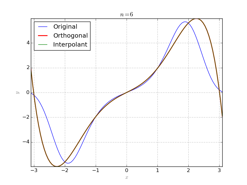
\(L^2\)-approximation with discrete measures
Suppose that \(\mu=\sum_1^n\delta_{x_i}\) is a measure with n-points in its support. Then the orthogonal system of polynomials consists of at most n+1 polynomials. Approximation with these n+1 polynomials is essentially same as interpolation:
# symbolic variable
x = Symbol('x')
# function to be approximated
g = sin(x)*exp(sin(x)*x)#x*sin(x)
# its numerical equivalent
g_ = lambdify(x, g, 'numpy')
# number of approximation terms
n = 6
# half interval length
l = 3.1
# interpolation points and values
Xs = [[-3], [-2], [-1], [0], [1], [2], [3]]
Ys = [g_(Xs[i][0]) for i in range(7)]
# a discrete measure
supp = {-3:1, -2:1, -1:1, 0:1, 1:1, 2:1, 3:1}
M = Measure(supp)
# orthogonal system
S = OrthSystem([x], [(-l, l)])
# link the measure
S.SetMeasure(M)
# polynomial basis
B = S.PolyBasis(n)
# link the basis to the orthogonal system
S.Basis(B)
# form the orthonormal basis
S.FormBasis()
# calculate coefficients
cfs = S.Series(g)
# orthogonal approximation
aprx = sum([S.OrthBase[i]*cfs[i] for i in range(len(B))])
# interpolate
Intrp = Interpolation([x])
intr = Intrp.Interpolate(Xs, Ys)
# plot the results
G = Graphics('sympy', numpoints=100)
G.SetTitle("$n = %d$"%(n))
G.Plot2D(g, (x, -l, l), color='blue', legend='Original')
G.Plot2D(aprx, (x, -l, l), color='red', legend='Orthogonal', thickness=2)
G.Plot2D(intr, (x, -l, l), color='green', legend='Interpolant')
G.save('OrthIntrp.png')