Hilbert Spaces¶

Orthonormal system of functions¶

Let X be a topological space and \(\mu\) be a finite Borel measure on X. The bilinear function \(\langle\cdot,\cdot\rangle\) defined on \(L^2(X, \mu)\) as \(\langle f, g\rangle = \int_X fg d\mu\) is an inner product which turns \(L^2(X, \mu)\) into a Hilbert space.

Let us denote the family of all continuous real valued functions on a non-empty compact space X by \(\textrm{C}(X)\). Suppose that among elements of \(\textrm{C}(X)\), a subfamily A of functions are of particular interest. Suppose that A is a subalgebra of \(\textrm{C}(X)\) containing constants. We say that an element \(f\in\textrm{C}(X)\) can be approximated by elements of A, if for every \(\epsilon>0\), there exists \(p\in A\) such that \(|f(x)-p(x)|<\epsilon\) for every \(x\in X\). The following classical results guarantees when every \(f\in\textrm{C}(X)\) can be approximated by elements of A.

Note

Stone-Weierstrass:

Every element of \(\textrm{C}(X)\) can be approximated by elements of A if and only if for every \(x\neq y\in X\), there exists \(p\in A\) such that \(p(x)\neq p(y)\).

Despite the strong and important implications of the Stone-Weierstrass theorem, it leaves every computational details out and does not give an specific algorithm to produce an estimator for f with elements of A, given an error tolerance \(\epsilon\), and the search for a such begins.

Define \(\|f\|_{\infty}\) (the \(\sup\) norm of f) of a given function \(f\in\textrm{C}(X)\) by

\[\|f\|_{\infty} = \sup_{x\in X}|f(x)|,\]

Then the above argument can be read as: For every \(f\in\textrm{C}(X)\) and every \(\epsilon>0\), there exists \(p\in A\) such that \(\|f-p\|_{\infty}<\epsilon\).

Let \((V, \langle\cdot,\cdot\rangle)\) be an inner product space with \(\|v\|_2=\langle v,v\rangle^{\frac{1}{2}}\). A basis \(\{v_{\alpha}\}_{\alpha\in I}\) is called an orthonormal basis for V if \(\langle v_{\alpha},v_{\beta}\rangle=\delta_{\alpha\beta}\), where \(\delta_{\alpha\beta}=1\) if and only if \(\alpha=\beta\) and is equal to 0 otherwise. Every given set of linearly independent vectors can be turned into a set of orthonormal vectors that spans the same sub vector space as the original. The following well-known result gives an algorithm for producing such orthonormal from a set of linearly independent vectors:

Note

Gram–Schmidt

Let \((V,\langle\cdot,\cdot\rangle)\) be an inner product space. Suppose \(\{v_{i}\}^{n}_{i=1}\) is a set of linearly independent vectors in V. Let

\[u_{1}:=\frac{v_{1}}{\|v_{1}\|_2}\]

and (inductively) let

\[w_{k}:=v_{k}-\sum_{i=1}^{k-1}\langle v_{k},u_{i}\rangle u_{i}\textrm{ and } u_{k}:=\frac{w_{k}}{\|w_{k}\|_2}.\]

Then \(\{u_{i}\}_{i=1}^{n}\) is an orthonormal collection, and for each k,

\[span\{u_{1},u_{2},\cdots,u_{k}\}=span\{v_{1},v_{2},\cdots,v_{k}\}.\]

Note that in the above note, we can even assume that \(n=\infty\).

Let \(B=\{v_1, v_2, \dots\}\) be an ordered basis for \((V,\langle\cdot,\cdot\rangle)\). For any given vector \(w\in V\) and any initial segment of B, say \(B_n=\{v_1,\dots,v_n\}\), there exists a unique \(v\in\textrm{span}(B_n)\) such that \(\|w-v\|_2\) is the minimum:

Note

Let \(w\in V\) and B a finite orthonormal set of vectors (not necessarily a basis). Then for \(v=\sum_{u\in B}\langle u,w\rangle u\)

\[\|w-v\|_2 = \min_{z\in\textrm{span}(B)}\|w-z\|_2.\]

Now, let \(\mu\) be a finite measure on X and for \(f,g\in\textrm{C}(X)\) define \(\langle f,g\rangle=\int_Xf g d\mu\). This defines an inner product on the space of functions. The norm induced by the inner product is denoted by \(\|\cdot\|_{2}\). It is evident that

\[\|f\|_{2}\leq\|f\|_{\infty}\mu(X),~\forall f\in\textrm{C}(X),\]

which implies that any good approximation in \(\|\cdot\|_{\infty}\) gives a good \(\|\cdot\|_{2}\)-approximation. But generally, our interest is the other way around. Employing Gram-Schmidt procedure, we can find \(\|\cdot\|_{2}\) within any desired accuracy, but this does not guarantee a good \(\|\cdot\|_{\infty}\)-approximation. The situation is favorable in finite dimensional case. Take \(B=\{p_1,\dots,p_n\}\subset\textrm{C}(X)\) and \(f\in\textrm{C}(X)\), then there exists \(K_f>0\) such that for every \(g\in\textrm{span}(B\cup\{f\})\),

\[K_f\|g\|_{\infty}\leq\|g\|_{2\leq}\|g\|_{\infty}\mu(X).\]

Since X is assumed to be compact, \(\textrm{C}(X)\) is separable, i.e., \(\textrm{C}(X)\) admits a countable dimensional dense subvector space (e.g. polynomials for when X is a closed, bounded interval). Thus for every \(f\in\textrm{C}(X)\) and every \(\epsilon>0\) one can find a big enough finite B, such that the above inequality holds. In other words, good enough \(\|\cdot\|_{2}\)-approximations of f give good \(\|\cdot\|_{\infty}\)-approximations, as desired.

OrthSystem¶

Given a measure space, the OrthSystem class implements the described procedure, symbolically. Therefore, it relies on a symbolic environment. Currently, three such environments are acceptable:

sympy

sage

symengine

Legendre polynomials¶

Let \(d\mu(x) = dx\), the regular Lebesgue measure on \([-1, 1]\) and \(B=\{1, x, x^2, \dots, x^n\}\). The orthonormal polynomials constructed from B are called Legendre polynomials. The \(n^{th}\) Legendre polynomial is denoted by \(P_n(x)\).

The following code generates Legendre polynomials up to a given order:

# the symbolic package
from sympy import *
from pyProximation import Measure, OrthSystem
# the symbolic variable
x = Symbol('x')
# set a limit to the order
n = 6
# define the measure
D = [(-1, 1)]
M = Measure(D, 1)
S = OrthSystem([x], D, 'sympy')
# link the measure to S
S.SetMeasure(M)
# set B = {1, x, x^2, ..., x^n}
B = S.PolyBasis(n)
# link B to S
S.Basis(B)
# generate the orthonormal basis
S.FormBasis()
# print the result
print B.OrthBase

Chebyshev polynomials¶

Let \(d\mu(x)=\frac{dx}{\sqrt{1-x^2}}\) on \([-1, 1]\) and B as in Legendre polynomials. The orthonormal polynomials associated to this setting are called Chebyshev polynomials and the \(n^{th}\) one is denoted by \(T_n(x)\).

The following code generates Chebyshev polynomials up to a given order:

# the symbolic package
from sympy import *
from numpy import sqrt
from pyProximation import Measure, OrthSystem
# the symbolic variable
x = Symbol('x')
# set a limit to the order
n = 6
# define the measure
D = [(-1, 1)]
w = lambda x: 1./sqrt(1. - x**2)
M = Measure(D, w)
S = OrthSystem([x], D, 'sympy')
# link the measure to S
S.SetMeasure(M)
# set B = {1, x, x^2, ..., x^n}
B = S.PolyBasis(n)
# link B to S
S.Basis(B)
# generate the orthonormal basis
S.FormBasis()
# print the result
print S.OrthBase

Approximation¶

Let \((X, \mu)\) be a compact Borel measure space and \(\mathcal{O}=\{u_1, u_2,\dots\}\) an orthonormal basis of function whose span is dense in \(L^2(X, \mu)\). Given a function \(f\in L^2(X, \mu)\), then f can be approximated as

\[f = \lim\limits_{n\rightarrow\infty}\sum_{i=1}^n\langle f, u_i\rangle u_i\]

OrthSystem.Series calculates the coefficients \(\langle f, u_i\rangle\):

Truncated Fourier series¶

Let \(d\mu(x) = dx\), the regular Lebesgue measure on \([c, c + 2l]\) and \(B=\{1, \sin(\pi x), \cos(\pi x), \sin(2\pi x), \cos(2\pi x), \dots, \sin(n\pi x), \cos(n\pi x),\}\). The following code calculates the Fourier series approximation of \(f(x)=\sin(x)e^x\):

from sympy import *
from numpy import sqrt
from pyProximation import Measure, OrthSystem
# the symbolic variable
x = Symbol('x')
# set a limit to the order
n = 4
# define the measure
D = [(-1, 1)]
w = lambda x: 1./sqrt(1. - x**2)
M = Measure(D, w)
S = OrthSystem([x], D, 'sympy')
# link the measure to S
S.SetMeasure(M)
# set B = {1, x, x^2, ..., x^n}
B = S.FourierBasis(n)
# link B to S
S.Basis(B)
# generate the orthonormal basis
S.FormBasis()
# number of elements in the basis
m = len(S.OrthBase)
# set f(x) = sin(x)e^x
f = sin(x)*exp(x)
# extract the coefficients
Coeffs = S.Series(f)
# form the approximation
f_app = sum([S.OrthBase[i]*Coeffs[i] for i in range(m)])
print f_app

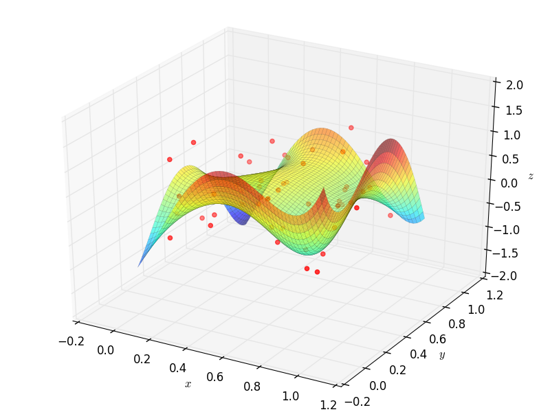
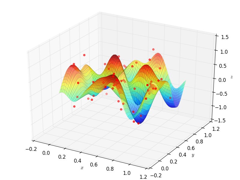
Fitting Data¶

Suppose that a set of data points \((x_1,y_1),\dots,(x_m,y_m)\) are given, where \(x_i\in\mathbb{R}^n\). To fit a curve or surface to data with minimum average square error, one can employ OrthSystem with an arbitrary system of functions to do so. The following example generates random data and fits two surfaces using polynomials and trigonometric functions:

from random import uniform
from sympy import *
from sympy.utilities.lambdify import lambdify, implemented_function
# import the module
from pyProximation import Measure, OrthSystem, Graphics
x, y, z = symbols('x, y, z')
# define dirac function symbolically and numerically
dirac = implemented_function(
    Function('dirac'), lambda a, b: 1 * (abs(a - b) < .000001))
# list of random points
points = [(uniform(0, 1), uniform(0, 1)) for _ in range(50)]
# container for the support of discrete measure
D = {}
# a symbolic function to represent the random points
g = 0
# Random values of the function
vals = []
for p in points:
    t = uniform(-.8, 1)
    vals.append(t)
    g += t * dirac(x, p[0]) * dirac(y, p[1])
    D[p] = 1
# The discrete measure supported at random points
M = Measure(D)
# Orthonormal systems of functions
S1 = OrthSystem([x, y], [(0, 1), (0, 1)])
S1.SetMeasure(M)

S2 = OrthSystem([x, y], [(0, 1), (0, 1)])
S2.SetMeasure(M)
# polynomial basis
B1 = S1.PolyBasis(4)
# trigonometric basis
B2 = S2.FourierBasis(3)
# link the basis to the orthogonal systems
S1.Basis(B1)
S2.Basis(B2)
# form the orthonormal basis
S1.FormBasis()
S2.FormBasis()
# calculate coefficients
cfs1 = S1.Series(g)
cfs2 = S2.Series(g)
# orthogonal approximation
aprx1 = sum([S1.OrthBase[i] * cfs1[i] for i in range(len(S1.OrthBase))])
aprx2 = sum([S2.OrthBase[i] * cfs2[i] for i in range(len(S2.OrthBase))])
# the graphic object
G1 = Graphics('sympy')
G2 = Graphics('sympy')
G1.Plot3D(aprx1, (x, 0, 1), (y, 0, 1))
G2.Plot3D(aprx2, (x, 0, 1), (y, 0, 1))
P = []
idx = 0
for p in points:
    q = (p[0], p[1], vals[idx])
    P.append(q)
    idx += 1
# link the points to the object
G1.Point(P, color='red')
G2.Point(P, color='red')
# save to file
G1.save('poly.png')
G2.save('trig.png')

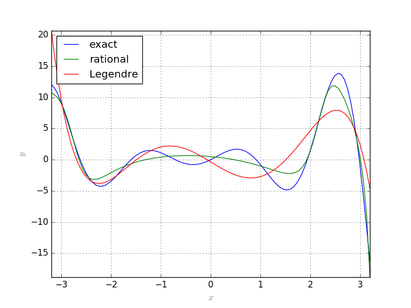
Rational Approximation¶

Let \(f:X\rightarrow\mathbb{R}\) be a continuous function and \(\{b_0, b_1,\dots\}\) an orthonormal system of functions over \(X\) with respect to a measure \(\mu\). Suppose that we want to approximate \(f\) with a function of the form \(\frac{p(x)}{q(x)}\) where \(p=\sum_{j=0}^m\alpha_jb_j\) and \(q=1+\sum_{j=1}^n\beta_jb_j\). Let \(r(x)=p(x)-q(x)f(x)\) be the residual. We can find the coefficients \(\alpha_i, \beta_j\) such that \(\|r\|_2\) be minimum.

Let \(L(\alpha, \beta)=r(x)\cdot r(x)\). Then the solution satisfies the following equations:

\[\begin{split}\frac{\partial}{\partial \alpha_i}L = 0,\\ \frac{\partial}{\partial \beta_i}L = 0,\end{split}\]

which is a system of linear equations. This is implemented in rational.RationalAprox.RatLSQ:

from sympy import *
from pyProximation import *

x = Symbol('x')
f = sinh(x) * cos(3 * x) + sin(3 * x) * exp(x)
D = [(-pi, pi)]
S = OrthSystem([x], D)
B = S.PolyBasis(5)

# link B to S
S.Basis(B)

# generate the orthonormal basis
S.FormBasis()

# extract the coefficients of approximations
Coeffs = S.Series(f)

# form the approximation
h = sum([S.OrthBase[i] * Coeffs[i] for i in range(len(S.OrthBase))])
T = RationalAprox(S)
g = T.RatLSQ(5, 5, f)

G = Graphics('sympy', 100)
G.Plot2D(f, (x, -3.2, 3.2), legend='exact')
G.Plot2D(g, (x, -3.2, 3.2), color='green', legend='rational')
G.Plot2D(h, (x, -3.2, 3.2), color='red', legend='Legendre')
G.save('Exm05.png')

Table of Contents

Previous topic

Next topic

This Page

Hilbert Spaces¶

Orthonormal system of functions¶

OrthSystem¶

Legendre polynomials¶

Chebyshev polynomials¶

Approximation¶

Truncated Fourier series¶

Fitting Data¶

Rational Approximation¶